

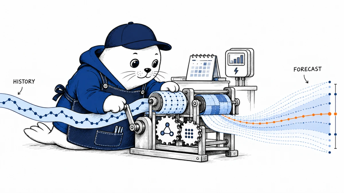
Most forecasting projects begin by training one model for one dataset. IBM’s new Granite release asks a cheaper first question: can a general pretrained model produce a useful forecast before you fit anything?
IBM released Granite Time Series PatchTST-FM-r2 on September 9, 2026. The open model makes zero-shot forecasts from recent history, returns uncertainty quantiles and can impute missing values. This model-card review separates the useful specifications from the leaderboard claim.
Model card: the numbers that shape deployment
| Model | IBM Granite Time Series PatchTST-FM-r2 |
|---|---|
| Parameters | Approximately 385 million |
| Training context | Up to 8,192 time steps |
| Patch design | Length 16, stride 8, 50% overlap |
| Forecast output | Point forecast plus a 99-quantile head |
| Licenses | Choose Apache 2.0 or OpenMDW 1.0 |
| Code | Weights, architecture, pipeline and benchmark materials published |
The architecture gives local and long-range patterns different jobs
IBM replaced the prior version’s plain transformer blocks with 30 conformer-style blocks. Each combines self-attention with temporal convolution. The intended division of labor is sensible: convolution captures nearby relationships, while attention can spend more capacity on distant dependencies.
The model also uses overlapping patches, Hamming-window weighting and overlap-and-add inference. Those choices are designed to reduce discontinuities where forecast patches meet. They are technical details with a visible product consequence: smoother forecasts across long horizons.
The 99 quantiles are more useful than one confident line
A point forecast says what the model expects. A quantile forecast describes a distribution of plausible values. That lets an inventory team estimate stockout risk, an energy operator plan for an upper-load range or an infrastructure team scale against a high CPU-utilization percentile.
Do not assume those intervals are calibrated on your data. Check how often the actual value lands below the predicted 10th, 50th and 90th percentiles. A useful interval should match its stated coverage over time and across seasonal regimes.
The leaderboard claim has a reproducibility footnote
IBM reports that PatchTST-FM-r2 ranks second on GIFT-Eval for CRPS and MASE among replicable, zero-shot models without test leakage. It reports geometric-mean scores of 0.467 CRPS and 0.6846 MASE, where lower is better. IBM also calls it the highest-performing model in that slice with a permissive commercial-friendly license.
The model card says the result is in a pending pull request to the GIFT-Eval benchmark. That means readers should treat the ranking as IBM-reported until the benchmark maintainers merge and display it. The narrower filtered slice also should not be converted into a claim that this is the best forecasting model for every task.
The training-data disclosure helps a real review
IBM lists four pretraining sources: selected GiftEvalPretrain datasets, custom KernelSynth-derived data, a TSMixup corpus excluding GIFT-Eval evaluation datasets, and about 500,000 synthetic CauKer sequences of length 4,096. That disclosure does not rule out every form of overlap, but it gives evaluators a concrete starting point.
The dual license is similarly practical. Users may choose Apache 2.0 or OpenMDW 1.0. The repository also warns that IBM provides the code as an open-source project without a commitment to maintenance, quality or security. Open weights reduce access friction; they do not outsource operational ownership.
A ten-minute trial can reject a bad fit
pip install "granite-tsfm>=0.3.9"

from tsfm_public import PatchTSTFMForPrediction
model = PatchTSTFMForPrediction.from_pretrained(
    "ibm-granite/granite-timeseries-patchtst-fm-r2"
)
Start with a chronological holdout from your own series. Compare r2 against a seasonal naive baseline and the current production model. Score both point error and quantile calibration, then segment failures by forecast horizon, missing-data pattern and regime change.
Our TimesFM 3 analysis is the obvious comparison because it separates model quality from production licensing. The BigQuery TabFM guide shows the opposite deployment tradeoff: managed SQL convenience instead of locally controlled open weights.
Use it first when the baseline is the bottleneck
- Good first fit: many related forecasting tasks where training and maintaining one model per series is expensive.
- Promising fit: demand, energy, telemetry or traffic workloads that benefit from uncertainty intervals.
- Needs caution: irregularly sampled events, abrupt policy changes or tasks where exogenous variables drive most of the signal.
- Production gate: beat a simple seasonal baseline on held-out data and remain calibrated across the regimes that matter.
My take: open zero-shot forecasting is becoming a baseline, not a bet
The most useful way to evaluate IBM Granite time series is not to ask whether one benchmark crowns it. Ask whether an openly inspectable 385M-parameter model can give your team a strong baseline before a custom training project begins. If it fails, you learn quickly. If it succeeds, the saved maintenance work may matter more than the leaderboard position.
Primary sources
- IBM release article and benchmark discussion
- IBM model card and weights
- Granite TSFM source repository
Checked September 13, 2026. Rankings and scores are attributed to IBM, and the model card says its GIFT-Eval result was pending benchmark merge. MustHave.ai has not independently rerun the evaluation.