

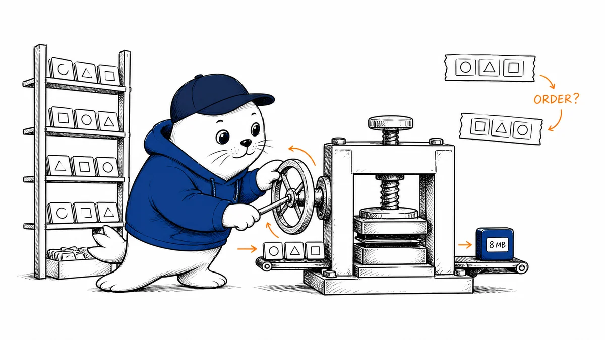
Lattice makes a retrieval model small by removing the expensive part. Instead of running a transformer over every sentence, it looks up one vector per token, averages the vectors, and normalizes the result.
That shortcut is why the Lattice static retriever can fit a 512-dimensional int4 deployment artifact into 7.94 MB. It is also why the model cannot understand word order, polysemy, or compositional meaning the way a contextual encoder can.
I ran the public checkpoint and the project’s slicer before writing this. The model returned normalized 1,024-dimensional embeddings, and the official conversion path produced the claimed 7.94 MB int4-row artifact. I did not reproduce the author’s full-Wikipedia speed run, so that number remains clearly attributed.
Why a lookup table can outrun an encoder
The full Lattice model is a 30,522 by 1,024 embedding table. For each input, the runtime tokenizes the text, retrieves the corresponding rows, mean-pools them, and applies L2 normalization. There is no attention layer deciding that the word "bank" means a river edge in one sentence and a financial institution in another.
That simplicity moves the bottleneck. In the author’s English Wikipedia run, tokenization consumed 91.7% of the wall time. The model math was no longer the expensive step.
The useful mental model: Lattice is a learned bag-of-tokens retriever, not a tiny transformer pretending to be one.
The training scale is still large. The author reports roughly 660 million curated query-document pairs, followed by hard-negative fine-tuning. Small inference does not mean small training.
What I reproduced locally
| Check | Result | Status |
|---|---|---|
| Public checkpoint load | Loaded erikkaum/lattice-retrieval with Sentence Transformers 5.4+. | Reproduced |
| Embedding shape | Three test strings returned a 3 × 1,024 matrix. | Reproduced |
| Normalization | All three vector norms were 1.0 to six decimal places. | Reproduced |
| Deployment artifact | The official slicer created a 512-dimensional int4-row file reported as 7.94 MB. | Reproduced |
| Wikipedia throughput | 6.4 million articles in 7 minutes 26 seconds on an 8-core Apple M2 MacBook Air. | Author-reported |
The local three-string encode took 0.243 seconds after the model loaded. That is a smoke test, not a throughput benchmark. Different hardware, warm-up, batching, text length, tokenizer cost, thread count, and output writes would make a direct comparison misleading.
The repository commit inspected for this check was fe4b29d. The checked-in evaluation JSON reports 0.469662 NDCG@10 for the 12-task decontaminated BEIR mean at 512 dimensions with int4-row quantization.
The quality loss is small on the reported mean, and specific to the test
The full 1,024-dimensional model reached 0.4749 NDCG@10 after fine-tuning. The 512-dimensional int4-row deployment variant scored 0.4697. That is an absolute difference of 0.0052, or roughly 1.1% relative to the full score.
Do not call that a pure quantization penalty. The deployment variant changes both precision and dimensionality. The number also averages twelve retrieval tasks; a workload with different language, domain, document length, or relevance judgments can move differently.
This is the same reason our endpoint accuracy analysis separates a published aggregate from the system you will actually run. Reproduce the operating point that matters to your product.
The shortcut breaks when order carries meaning
Mean-pooling token vectors ignores order. "The dog bites the man" and "the man bites the dog" contain nearly the same tokens, so a static retriever has no sequence mechanism that can reliably preserve the reversal.
- Word order: instructions, negation, and subject-object relationships can collapse toward similar vectors.
- Polysemy: one token keeps one learned row even when its meaning changes with context.
- Compositional meaning: the model can learn useful aggregate associations, but it does not build a contextual representation through attention.
- Language scope: the release is an English retriever; multilingual coverage should not be assumed.
Those limitations do not make the model useless. They define the jobs it should and should not own.
Where Lattice fits in a retrieval stack
| Need | Best starting point | Why |
|---|---|---|
| Offline or on-device candidate generation | Lattice | Tiny artifact, CPU-friendly runtime, no remote inference dependency. |
| Very large corpus, cheap first pass | Lattice plus reranker | Use speed for recall, then spend context on a small candidate set. |
| Negation, order, or nuanced instructions | Contextual encoder | Attention can represent relationships that mean pooling drops. |
| High-consequence retrieval | Hybrid search plus evaluation | Combine lexical and semantic evidence, then test misses and false positives. |
The strongest use is probably not "replace every embedding model." It is "make the first pass cheap enough to run everywhere." A static retriever can generate candidates locally, while a contextual model or reranker handles the ambiguous tail.
If you are choosing between this and an API, our guide to open weights versus closed APIs covers the operational trade. Our model selection framework adds the missing question: what happens when retrieval is wrong?
My verdict: buy speed with a second stage
Lattice is an unusually honest engineering trade. It does not make contextual retrieval magically free. It removes context from the first-stage model, trains the remaining lookup table very hard, and exposes the result through a small Rust runtime.
Use it when memory, CPU cost, offline operation, or indexing speed is the constraint. Keep a contextual reranker, lexical path, or human review where word order and nuance decide the answer.
Read and reproduce the source
- Read the author’s Lattice engineering write-up.
- Inspect the public Lattice repository and evaluation files.
- Download the Lattice retrieval checkpoint.
Would you trade contextual understanding for a first-stage retriever small enough to ship inside your product?
Checked August 9, 2026. Model architecture, training scale, evaluation results, and Wikipedia throughput come from the author’s public model card, write-up, repository, and checked-in evaluation files. Musthave.ai independently loaded the checkpoint, checked normalized output shape, and generated the 7.94 MB int4-row artifact. The 1.1% figure is the relative difference between 0.4749 and 0.4697; it combines dimension reduction and quantization.